Customizing Plots
Almost every visual aspect of a plot can be changed at runtime with keyword arguments. Any line you type at the prompt that contains key=value pairs is applied to the current plot.
CDFViewer> title="Air temperature", xlabel="Longitude", ylabel="Latitude"
┌ Info: Current plot settings:
│ title => "Air temperature"
│ xlabel => "Longitude"
└ ylabel => "Latitude"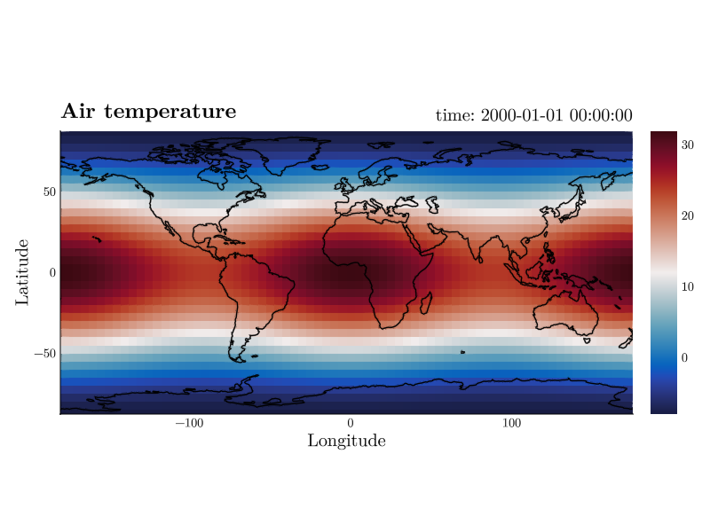
Values are parsed as Julia expressions. :thermal is a symbol, (-20, 30) a tuple, "Air temperature" a string. Multiple pairs are separated by commas.
Function calls count as expressions too, module prefix included. A keyword that wants an object rather than a number is written the way you would write it in Julia, for example colorscale=Makie.Symlog10(1e-2) for a symmetric log color scale, or color=RGBf(1, 0, 0). Makie, Colors and Dates are in scope. A bare word stays a string, so title=Temperature needs no quotes. A call that fails to evaluate is reported on the terminal and the keyword keeps its previous value.
Where the keywords go
You never have to say what a keyword belongs to. CDFViewer routes each one automatically to the figure, the axis, the plot object, the colorbar, or the interpolation ranges, whichever accepts it. The kwargs command lists what is available, grouped by these categories.
CDFViewer> kwargs figure
CDFViewer> kwargs axis
CDFViewer> kwargs plot
CDFViewer> kwargs colorbar
CDFViewer> kwargs range
Since the available keywords depend on the current plot type, the lists are long. Try them in a running session (TAB completion works on keyword names, too).
Colormap and color range
colormap accepts any Makie colormap name, and colorrange pins the color scale, which is useful to compare different time steps on the same scale or before recording an animation.
CDFViewer> colormap=:thermal, colorrange=(-20, 30)
┌ Info: Current plot settings:
│ title => "Air temperature"
│ xlabel => "Longitude"
│ ylabel => "Latitude"
│ colormap => :thermal
└ colorrange => (-20, 30)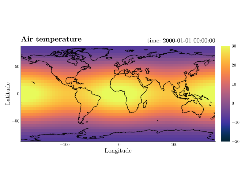
The colorbar follows automatically. During animation the range is pinned on its own for reasonably sized variables, and colorrange also accepts the modes "cycle", "data", and "frame" to control that (see Stable colors during playback). Deleting the keyword (del colorrange) returns to the default pinning.
Labelling the colorbar
The colorbar starts without a label. cbarlabel="auto" labels it with the variable's name and unit – the string the figure title uses by default – and the label follows when you switch variables. Any other string is drawn as given. On a vector plot, where the colors are a magnitude, "auto" names that magnitude instead (see Plot Types).
CDFViewer> cbarlabel="auto"
┌ Info: Current plot settings:
│ title => "Air temperature"
│ xlabel => "Longitude"
│ ylabel => "Latitude"
│ colormap => :thermal
│ colorrange => (-20, 30)
└ cbarlabel => "auto"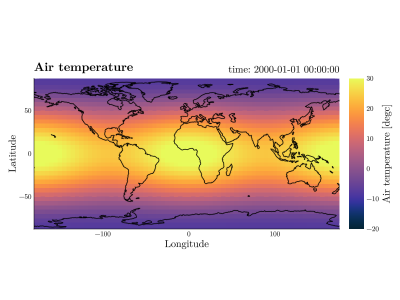
cbarlabelsize, cbarlabelcolor, cbarlabelfont, cbarlabelrotation (in radians, automatic by default) and cbarlabelpadding style it. cbarlabel=false or del cbarlabel takes it away again.
CDFViewer> del cbarlabel
┌ Info: Current plot settings:
│ title => "Air temperature"
│ xlabel => "Longitude"
│ ylabel => "Latitude"
│ colormap => :thermal
└ colorrange => (-20, 30)
Contour levels and labels
Plot-specific keywords work the same way. A contour plot, for example, takes the levels to draw – a number of them, a range, or a list of the values themselves – and can label them directly on the lines.
CDFViewer> p contour
[ Info: Selected: contour
CDFViewer> levels=-30:5:30, labels=true
┌ Info: Current plot settings:
│ title => "Air temperature"
│ xlabel => "Longitude"
│ ylabel => "Latitude"
│ colormap => :thermal
│ colorrange => (-20, 30)
│ levels => -30:5:30
└ labels => true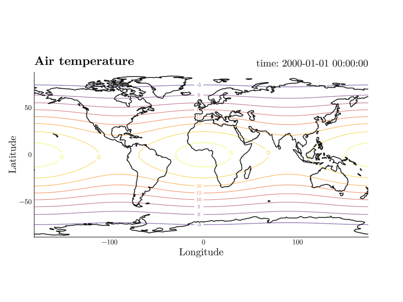
Inspecting and resetting
get shows the current value of a keyword, conf lists everything you have set, del removes keywords and restores their defaults, and reset clears all customizations at once.
CDFViewer> get colormap
[ Info: colormap => :thermal
CDFViewer> conf
┌ Info: Current plot settings:
│ title => "Air temperature"
│ xlabel => "Longitude"
│ ylabel => "Latitude"
│ colormap => :thermal
│ colorrange => (-20, 30)
│ levels => -30:5:30
└ labels => true
CDFViewer> del labels levels
┌ Info: Current plot settings:
│ title => "Air temperature"
│ xlabel => "Longitude"
│ ylabel => "Latitude"
│ colormap => :thermal
└ colorrange => (-20, 30)
CDFViewer> reset
[ Info: Reset plot settings to default.
Figure settings
A few special keywords control the figure itself rather than the plot.
| Keyword | Default | Effect |
|---|---|---|
figsize=(800, 600) | (800, 600) | size of the figure in pixels |
titlesize=28 | 24 | fontsize of the figure title |
xunit="km" | (none) | render an axis in another unit (see Axis units) |
cbar=true | true | show or hide the colorbar |
cbarlabel="auto" | (none) | label the colorbar ("auto" takes the variable's label) |
cbarlabelsize=26 | 20 | fontsize of the colorbar label |
cbarlabelcolor=:red | :black | color of the colorbar label |
cbarlabelfont="bold" | "regular" | font of the colorbar label |
cbarlabelrotation=0 | (automatic) | rotation of the colorbar label in radians |
cbarlabelpadding=5 | 5 | gap between the bar and its label |
moveable=true | true | allow drag-panning with the mouse |
geographic=false | false | draw on a geographic map projection |
proj="+proj=moll" | (none) | map projection (PROJ string) |
scale=110 | 110 | coastline resolution in m (10, 50, or 110) |
coastlines=true | true | draw coastlines (geographic mode) |
land=false | false | fill land masses (geographic mode) |
earth=false | false | satellite image background (geographic mode) |
rotate=20 | 0 | orbit the 3D camera horizontally (degrees per second) |
rotatev=5 | 0 | move the 3D camera vertically, bouncing inside rotatevlim |
rotatelim=(-45, 45) | (none) | bound the orbit to an azimuth sector (back-and-forth sweep) |
rotatevlim=(0, 80) | (0, 80) | elevation range of the vertical bounce |
arrows=(24, 16) | (24, 16) | arrows per axis in a quiver plot |
every=4 | (none) | draw every n-th grid point instead (quiver) |
minspeed=9 | (none) | draw nothing slower than this (quiver, streamplot) |
lengthscale=40 | (none) | fixed arrow length, in pixels per unit speed (quiver) |
The label showing the current playback value is configured the same way, through its own animlabel... keywords (see Animation and Playback).
The shape of the plot box
A two-dimensional field is drawn in a box shaped like its own coordinates. A section 2400 m wide and 120 m deep comes out twenty times as wide as it is tall, so a one-in-twenty slope looks like one and a round eddy stays round. The box keeps that shape inside the figure instead of stretching to fill it, and the colorbar follows its height. A 3D axis does the same with its three edge lengths.
The window follows. 800 by 600 is a guess made before the file was ever opened, and a 20:1 section drawn true inside it is a thirty-pixel band adrift in an empty canvas. So when the data asks for a shape the default cannot hold, the window is opened shaped like the data instead: the same section comes up around 1600 by 190, with the box filling it and room for its ticks. You never have to ask for this, and it holds for --savefig and --record as much as on screen – which is the point, since a recorded plot gets no second chance at a window.
The shape is exact up to about 24:1. Past that a section is a line whatever window it is given – 6000 km across by 4 km deep cannot be drawn both true and readable at any size – so the ratio is held there and the box fills its window rather than thinning to a hairline inside it. That limit does not move with the figure, so a window of your own is never quietly redrawn at some other ratio.
figsize and aspect each override all of it outright. figsize=(1000, 400) fixes the window and stops one being chosen for you; aspect=1 gives a square box whatever the data says, and on a 3D axis aspect=(2, 1, 0.5) sets the three edge lengths. A window you resize by hand is yours as well, and is not resized under you afterwards.
Geographic plots
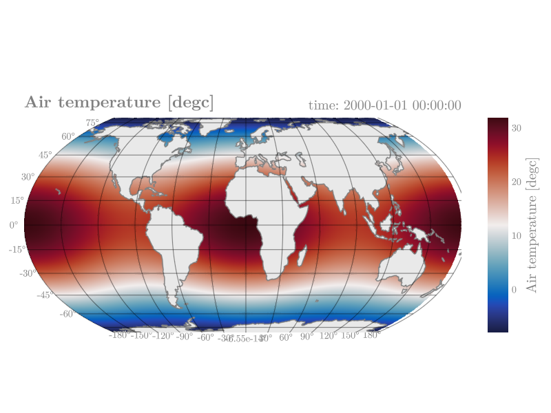
For 2D fields on longitude/latitude axes, geographic=true switches the axis to a map projection. heatmap, contour, contourf, quiver, and streamplot support it. The automatic longitude tick labels tend to bunch up at the curved map edge, so we hide them here with a regular axis keyword.
CDFViewer> geographic=true, land=true, xticklabelsvisible=false
┌ Info: Current plot settings:
│ geographic => true
│ land => true
└ xticklabelsvisible => false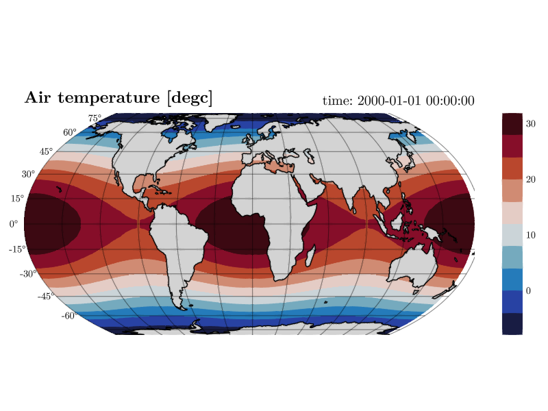
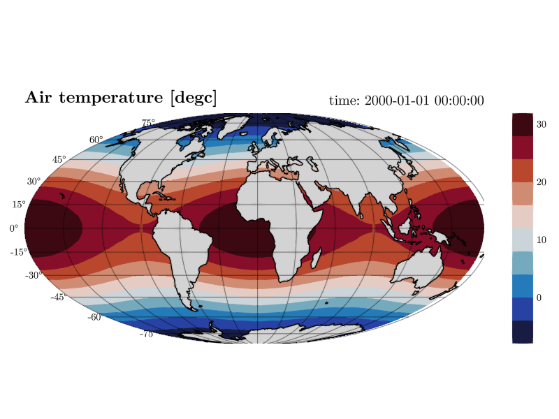
The projection can be any PROJ string, for example a Mollweide projection.
Axis units
Coordinates are often stored in base units such as meters or seconds, while the domain is better read in a larger one. A field spanning hundreds of kilometers draws meter ticks in scientific notation. The xunit, yunit, and zunit keywords render an axis in another unit of the same family.
CDFViewer> xunit="km", yunit="km"
┌ Info: Current plot settings:
│ xunit => "km"
└ yunit => "km"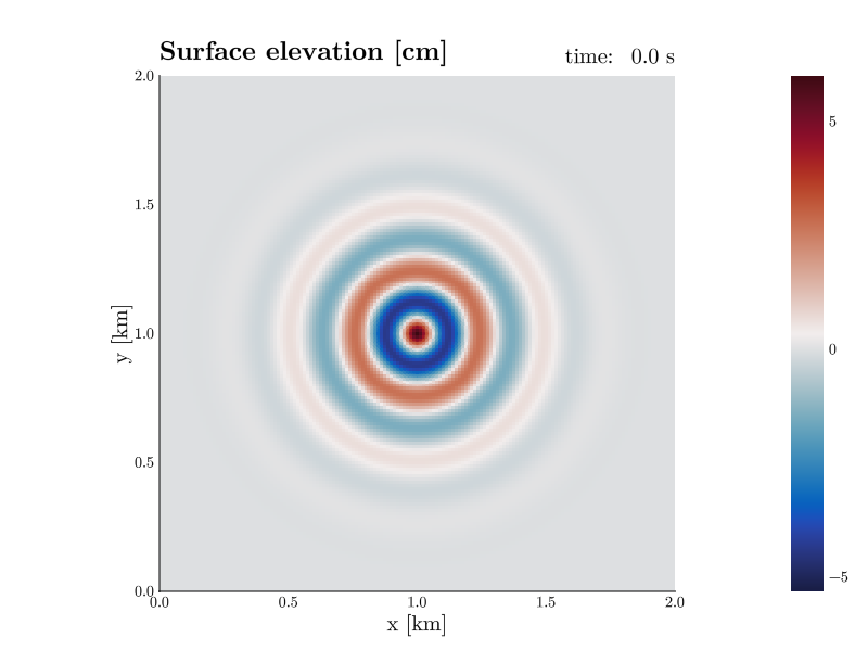
Tick values are chosen to be round in the displayed unit, and the axis label switches to it. Everything else stays in native coordinates. Axis limits, interpolation ranges, and the values shown by the data inspector are unaffected, because the conversion is purely visual.
Units convert only within their family.
| Family | Units |
|---|---|
| length | mm, cm, m, km |
| time | ns, µs, ms, s, min, h, d, yr |
| pressure | Pa, hPa, mbar, kPa, dbar, bar |
A year here is the Julian year of 365.25 days. Asking for a unit the axis cannot convert to (say xunit="bar" on a meter axis) keeps the native ticks and reports why. del xunit returns to the native unit.
The label naming the current playback value converts the same way through the animunit keyword (see Animation and Playback).
Themes
The whole figure can be drawn in another look. Pass --theme on the command line to start in one, or use the theme command to change it while the viewer runs.
CDFViewer> theme black
[ Info: Theme: black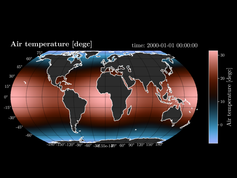
Five themes are available, all of them Makie's own: minimal (the default), light, dark, black, and ggplot2. theme without a name reports the one in use. Makie's own spelling is accepted as well, so theme theme_dark and theme dark mean the same thing.
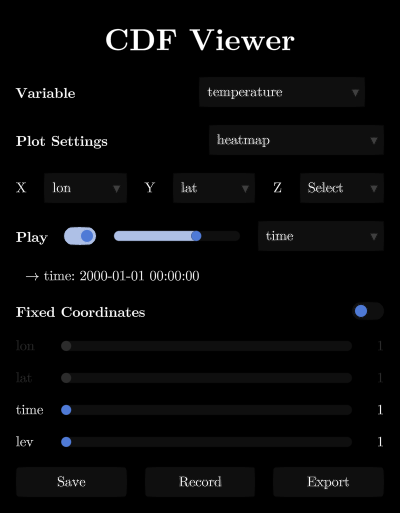
Everything CDFViewer draws itself follows the theme instead of assuming a white page: coastlines, the land fill, the colorbar label, the box behind the playback label, the contour lines of an overlay, and the whole of the menu window – the face of every button, dropdown, toggle and slider as much as the lettering on it. All of it is derived from the two colors every theme fixes, its background and its text color, so black coastlines never end up on a black background and a dropdown is never a white box on a dark page. The one thing that keeps its own color under every theme is the blue a widget lights up in when you point at it or drag it, which is Makie's and reads on either ground.
The colormap follows too. An untouched field is drawn in :balance, which is white in the middle, on a light page; on a dark page that white band would be the brightest thing on the figure, so a dark theme starts fields in :berlin instead – the same diverging shape with its pale band moved off the middle of the range and onto its ends. Only the starting point moves: a colormap= you set yourself outranks it and is put back after the switch, like every other keyword. The line color of a 1D plot is left alone, a mid-blue that reads on either ground.
A theme is not a keyword argument, because a figure takes its theme at the moment it is created and never looks at it again. Type theme=dark out of habit and the prompt hands you the command form back. theme therefore rebuilds both windows and puts the session back into them: the variable, the axes, the plot type, every slider position, the playback dimension, speed and state, all overlays, your keyword arguments, the save options, the figure size and the zoom. The windows keep their place on screen. The theme is also part of what export prints, so a session restarts in the look you left it in.
Dimensionless quantities
Some files mark a quantity as dimensionless rather than leaving the unit out, and CDFViewer prints no unit for those. The CF convention spells it units = "1", and dimensionless, none, -, and the empty string count as well, whatever the case and surrounding whitespace. Such a variable is labelled exactly like one carrying no units attribute at all, everywhere a unit appears: axis labels, the figure title, the playback readout, and the dataset overview. Units that only look similar keep printing, among them 1e-3, 1/s, and %.
Keyword arguments survive plot type switches where possible and can also be passed at startup with --kwargs='colormap=:viridis, ...' (see Command Line Options).